Note
Click here to download the full example code
Multi-subject joint source localization with multi-task models.
The aim of this tutorial is to show how to leverage functional similarity across subjects to improve source localization. For that purpose we use the the high frequency SEF MEG dataset of (Nurminen et al., 2017) which provides MEG and MRI data for two subjects.
# Author: Hicham Janati (hicham.janati@inria.fr)
#
# License: BSD (3-clause)

import mne
import os
import os.path as op
from mne.parallel import parallel_func
from mne.datasets import hf_sef
from matplotlib import pyplot as plt

from groupmne import group_model
from groupmne.inverse import compute_group_inverse
Download and process MEG data
For this example, we use the HF somatosensory dataset [2]. We need the raw data to estimate the noise covariance since only average MEG data (and MRI) are provided in “evoked”. The data will be downloaded in the same location
_ = hf_sef.data_path("raw")
data_path = hf_sef.data_path("evoked")
meg_path = data_path + "/MEG/"
data_path = op.expanduser(data_path)
subjects_dir = data_path + "/subjects/"
os.environ['SUBJECTS_DIR'] = subjects_dir
raw_name_s = [meg_path + s for s in ["subject_a/sef_right_raw.fif",
"subject_b/hf_sef_15min_raw.fif"]]
def process_meg(raw_name):
"""Extract epochs from a raw fif file.
Parameters
----------
raw_name: str.
path to the raw fif file.
Returns
-------
epochs: Epochs instance
"""
raw = mne.io.read_raw_fif(raw_name)
events = mne.find_events(raw)
event_id = dict(hf=1) # event trigger and conditions
tmin = -0.05 # start of each epoch (50ms before the trigger)
tmax = 0.3 # end of each epoch (300ms after the trigger)
baseline = (None, 0) # means from the first instant to t = 0
epochs = mne.Epochs(raw, events, event_id, tmin, tmax, proj=True,
baseline=baseline)
return epochs
epochs_s = [process_meg(raw_name) for raw_name in raw_name_s]
evoked_s = [ep.average() for ep in epochs_s]
# compute noise covariance (takes a few minutes)
noise_cov_s = []
for subj, ep in zip(["a", "b"], epochs_s):
cov_fname = meg_path + f"subject_{subj}/sef-cov.fif"
if os.path.exists(cov_fname):
cov = mne.read_cov(cov_fname)
else:
cov = mne.compute_covariance(ep, tmin=None, tmax=0.)
mne.write_cov(cov_fname, cov)
noise_cov_s.append(cov)
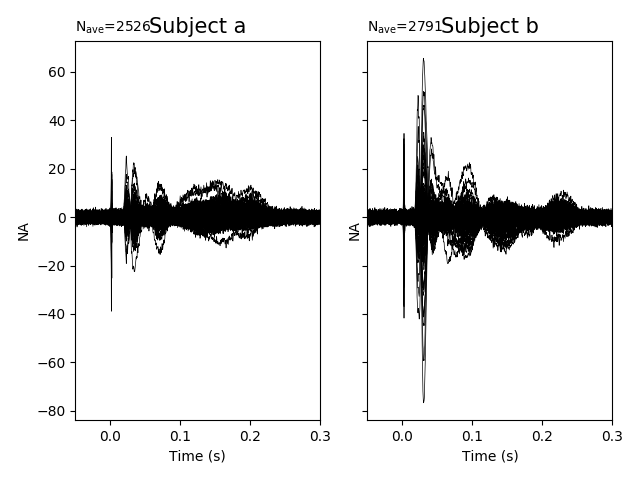
f, axes = plt.subplots(1, 2, sharey=True)
for ax, ev, nc, ll in zip(axes.ravel(), evoked_s, noise_cov_s, ["a", "b"]):
picks = mne.pick_types(ev.info, meg="grad")
ev.plot(picks=picks, axes=ax, noise_cov=nc, show=False)
ax.set_title("Subject %s" % ll, fontsize=15)
plt.show()
Out:
Opening raw data file /Users/hichamjanati/mne_data/HF_SEF/MEG/subject_a/sef_right_raw.fif...
    Read a total of 8 projection items:
        generated with autossp-1.0.1 (1 x 306)  idle
        generated with autossp-1.0.1 (1 x 306)  idle
        generated with autossp-1.0.1 (1 x 306)  idle
        generated with autossp-1.0.1 (1 x 306)  idle
        generated with autossp-1.0.1 (1 x 306)  idle
        generated with autossp-1.0.1 (1 x 306)  idle
        generated with autossp-1.0.1 (1 x 306)  idle
        generated with autossp-1.0.1 (1 x 306)  idle
    Range : 26000 ... 1735999 =      8.667 ...   578.666 secs
Ready.
Opening raw data file /Users/hichamjanati/mne_data/HF_SEF/MEG/subject_a/sef_right_raw-1.fif...
    Read a total of 8 projection items:
        generated with autossp-1.0.1 (1 x 306)  idle
        generated with autossp-1.0.1 (1 x 306)  idle
        generated with autossp-1.0.1 (1 x 306)  idle
        generated with autossp-1.0.1 (1 x 306)  idle
        generated with autossp-1.0.1 (1 x 306)  idle
        generated with autossp-1.0.1 (1 x 306)  idle
        generated with autossp-1.0.1 (1 x 306)  idle
        generated with autossp-1.0.1 (1 x 306)  idle
    Range : 1736000 ... 2482999 =    578.667 ...   827.666 secs
Ready.
Current compensation grade : 0
2527 events found
Event IDs: [1]
2527 matching events found
Applying baseline correction (mode: mean)
Not setting metadata
Created an SSP operator (subspace dimension = 8)
8 projection items activated
Opening raw data file /Users/hichamjanati/mne_data/HF_SEF/MEG/subject_b/hf_sef_15min_raw.fif...
    Read a total of 8 projection items:
        generated with autossp-1.0.1 (1 x 306)  idle
        generated with autossp-1.0.1 (1 x 306)  idle
        generated with autossp-1.0.1 (1 x 306)  idle
        generated with autossp-1.0.1 (1 x 306)  idle
        generated with autossp-1.0.1 (1 x 306)  idle
        generated with autossp-1.0.1 (1 x 306)  idle
        generated with autossp-1.0.1 (1 x 306)  idle
        generated with autossp-1.0.1 (1 x 306)  idle
    Range : 169000 ... 1878999 =     56.333 ...   626.333 secs
Ready.
Opening raw data file /Users/hichamjanati/mne_data/HF_SEF/MEG/subject_b/hf_sef_15min_raw-1.fif...
    Read a total of 8 projection items:
        generated with autossp-1.0.1 (1 x 306)  idle
        generated with autossp-1.0.1 (1 x 306)  idle
        generated with autossp-1.0.1 (1 x 306)  idle
        generated with autossp-1.0.1 (1 x 306)  idle
        generated with autossp-1.0.1 (1 x 306)  idle
        generated with autossp-1.0.1 (1 x 306)  idle
        generated with autossp-1.0.1 (1 x 306)  idle
        generated with autossp-1.0.1 (1 x 306)  idle
    Range : 1879000 ... 2892999 =    626.333 ...   964.333 secs
Ready.
Current compensation grade : 0
2792 events found
Event IDs: [1]
2792 matching events found
Applying baseline correction (mode: mean)
Not setting metadata
Created an SSP operator (subspace dimension = 8)
8 projection items activated
    306 x 306 full covariance (kind = 1) found.
    Read a total of 8 projection items:
        generated with autossp-1.0.1 (1 x 306) active
        generated with autossp-1.0.1 (1 x 306) active
        generated with autossp-1.0.1 (1 x 306) active
        generated with autossp-1.0.1 (1 x 306) active
        generated with autossp-1.0.1 (1 x 306) active
        generated with autossp-1.0.1 (1 x 306) active
        generated with autossp-1.0.1 (1 x 306) active
        generated with autossp-1.0.1 (1 x 306) active
Computing data rank from covariance with rank=None
    Using tolerance 2.6e-13 (2.2e-16 eps * 204 dim * 5.8  max singular value)
    Estimated rank (grad): 201
    GRAD: rank 201 computed from 204 data channels with 3 projectors
Computing data rank from covariance with rank=None
    Using tolerance 1.1e-14 (2.2e-16 eps * 102 dim * 0.48  max singular value)
    Estimated rank (mag): 97
    MAG: rank 97 computed from 102 data channels with 5 projectors
Computing data rank from covariance with rank=None
    Using tolerance 2.2e-13 (2.2e-16 eps * 204 dim * 4.9  max singular value)
    Estimated rank (grad): 201
    GRAD: rank 201 computed from 204 data channels with 3 projectors
Computing data rank from covariance with rank=None
    Using tolerance 5.2e-15 (2.2e-16 eps * 102 dim * 0.23  max singular value)
    Estimated rank (mag): 97
    MAG: rank 97 computed from 102 data channels with 5 projectors
Source and forward modeling
To guarantee an alignment across subjects, we start by computing (or reading if available) the source space of the average subject of freesurfer fsaverage If fsaverage is not available, it will be fetched to the data_path
resolution = 4
spacing = "ico%d" % resolution
src_ref = group_model.get_src_reference(spacing=spacing,
                                        subjects_dir=subjects_dir)
Out:
Setting up the source space with the following parameters:

SUBJECTS_DIR = /Users/hichamjanati/mne_data/HF_SEF/subjects/
Subject      = fsaverage
Surface      = white
Icosahedron subdivision grade 4

>>> 1. Creating the source space...

Doing the icosahedral vertex picking...
Loading /Users/hichamjanati/mne_data/HF_SEF/subjects/fsaverage/surf/lh.white...
Mapping lh fsaverage -> ico (4) ...
    Warning: zero size triangles: [3 4]
    Triangle neighbors and vertex normals...
Loading geometry from /Users/hichamjanati/mne_data/HF_SEF/subjects/fsaverage/surf/lh.sphere...
Setting up the triangulation for the decimated surface...
loaded lh.white 2562/163842 selected to source space (ico = 4)

Loading /Users/hichamjanati/mne_data/HF_SEF/subjects/fsaverage/surf/rh.white...
Mapping rh fsaverage -> ico (4) ...
    Warning: zero size triangles: [3 4]
    Triangle neighbors and vertex normals...
Loading geometry from /Users/hichamjanati/mne_data/HF_SEF/subjects/fsaverage/surf/rh.sphere...
Setting up the triangulation for the decimated surface...
loaded rh.white 2562/163842 selected to source space (ico = 4)

You are now one step closer to computing the gain matrix
the function group_model.compute_fwd morphs the source space src_ref to the surface of each subject by mapping the sulci and gyri patterns and computes their forward operators.
subjects = ["subject_a", "subject_b"]
trans_fname_s = [meg_path + "%s/%s-trans.fif" % (s, s) for s in subjects]
bem_fname_s = [subjects_dir + "%s/bem/%s-5120-bem-sol.fif" % (s, s)
               for s in subjects]
n_jobs = 2
parallel, run_func, _ = parallel_func(group_model.compute_fwd, n_jobs=n_jobs)

fwds = parallel(run_func(s, src_ref, info, trans, bem,  mindist=3)
                for s, info, trans, bem in zip(subjects, raw_name_s,
                                               trans_fname_s, bem_fname_s))
We can now compute the data of the inverse problem. group_info is a dictionary that contains the selected channels and the alignment maps between src_ref and the subjects which are required if you want to plot source estimates on the brain surface of each subject. The We restric the time points around 20ms in order to reconstruct the sources of the N20 response.
gains, M, group_info = \
    group_model.compute_inv_data(fwds, src_ref, evoked_s, noise_cov_s,
                                 ch_type="grad", tmin=0.015, tmax=0.025)
print("(# subjects, # channels, # sources) = ", gains.shape)
print("(# subjects, # channels, # time points) = ", M.shape)
Out:
No patch info available. The standard source space normals will be employed in the rotation to the local surface coordinates....
    Changing to fixed-orientation forward solution with surface-based source orientations...
    [done]
Mapping lh fsaverage -> subject_a (nearest neighbor)...
Mapping rh fsaverage -> subject_a (nearest neighbor)...
    No patch info available. The standard source space normals will be employed in the rotation to the local surface coordinates....
    Changing to fixed-orientation forward solution with surface-based source orientations...
    [done]
Mapping lh fsaverage -> subject_b (nearest neighbor)...
Mapping rh fsaverage -> subject_b (nearest neighbor)...
    Created an SSP operator (subspace dimension = 3)
Computing data rank from covariance with rank=None
    Using tolerance 2.6e-13 (2.2e-16 eps * 204 dim * 5.8  max singular value)
    Estimated rank (grad): 201
    GRAD: rank 201 computed from 204 data channels with 3 projectors
    Setting small GRAD eigenvalues to zero (without PCA)
    Created the whitener using a noise covariance matrix with rank 201 (3 small eigenvalues omitted)
    Created an SSP operator (subspace dimension = 3)
Computing data rank from covariance with rank=None
    Using tolerance 2.2e-13 (2.2e-16 eps * 204 dim * 4.9  max singular value)
    Estimated rank (grad): 201
    GRAD: rank 201 computed from 204 data channels with 3 projectors
    Setting small GRAD eigenvalues to zero (without PCA)
    Created the whitener using a noise covariance matrix with rank 201 (3 small eigenvalues omitted)
(# subjects, # channels, # sources) =  (2, 204, 5124)
(# subjects, # channels, # time points) =  (2, 204, 31)
Solve the inverse problems with groupmne
For now, only the group lasso model [1] is supported. It assumes the source locations are the same across subjects for all instants i.e if a source is zero for one subject, it will be zero for all subjects. “alpha” is a hyperparameter that controls this structured sparsity prior. it must be set as a positive number between 0 and 1. With alpha = 1, all the sources are 0.
stcs, log = compute_group_inverse(gains, M, group_info,
                                  method="grouplasso",
                                  depth=0.9, alpha=0.7, return_stc=True,
                                  n_jobs=4)
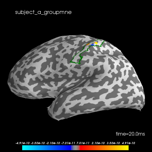
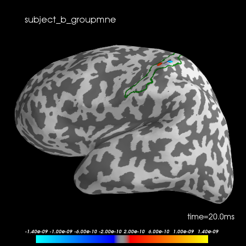
Let’s visualize the N20 response. The stimulus was applied on the right hand, thus we only show the left hemisphere. The activation is exactly in the Primary somatosensory cortex. We highlight the borders of the post central gyrus.
t = 0.02
t_idx = stcs[0].time_as_index(t)
view = "lateral"
for stc, subject in zip(stcs, subjects):
    g_post_central = mne.read_labels_from_annot(subject, "aparc.a2009s",
                                                subjects_dir=subjects_dir,
                                                regexp="G_postcentral-lh")[0]
    m = abs(stc.data[:group_info["n_sources"][0], t_idx]).max()
    surfer_kwargs = dict(
        clim=dict(kind='value', pos_lims=[0., 0.1 * m, m]),
        hemi='lh', subjects_dir=subjects_dir,
        initial_time=t * 1e3, time_unit='ms', size=(500, 500),
        smoothing_steps=5)
    brain = stc.plot(**surfer_kwargs, views=view)
    brain.add_text(0.1, 0.9, subject + "_groupmne", "title")
    brain.add_label(g_post_central, borders=True, color="green")
Out:
Reading labels from parcellation...
   read 1 labels from /Users/hichamjanati/mne_data/HF_SEF/subjects/subject_a/label/lh.aparc.a2009s.annot
   read 0 labels from /Users/hichamjanati/mne_data/HF_SEF/subjects/subject_a/label/rh.aparc.a2009s.annot
Reading labels from parcellation...
   read 1 labels from /Users/hichamjanati/mne_data/HF_SEF/subjects/subject_b/label/lh.aparc.a2009s.annot
   read 0 labels from /Users/hichamjanati/mne_data/HF_SEF/subjects/subject_b/label/rh.aparc.a2009s.annot
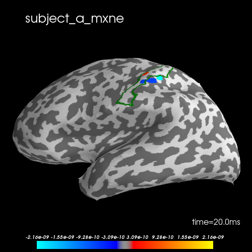
Group MNE leads to better accuracy
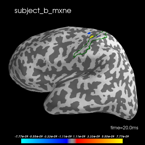
To evaluate the effect of the joint inverse solution, we compute the individual solutions using mne.inverse_sparse.mixed_norm for each subject. The group solutions are better located in S1.
from mne.inverse_sparse import mixed_norm  # noqa: E402

t = 0.02
t_idx = stcs[0].time_as_index(t)
view = "lateral"
for subject, evoked, fwd, cov in zip(subjects, evoked_s, fwds, noise_cov_s):
    ev = evoked.copy()
    ev.pick_types(meg="grad")
    ev.crop(0.015, 0.025)
    stc = mixed_norm(ev, fwd, cov, alpha=60., loose=0., depth=0.9)
    stc.subject = subject
    g_post_central = mne.read_labels_from_annot(subject, "aparc.a2009s",
                                                subjects_dir=subjects_dir,
                                                regexp="G_postcentral-lh")[0]
    m = abs(stc.data[:group_info["n_sources"][0], t_idx]).max()
    surfer_kwargs = dict(
        clim=dict(kind='value', pos_lims=[0., 0.1 * m, m]),
        hemi='lh', subjects_dir=subjects_dir,
        initial_time=t * 1e3, time_unit='ms', size=(500, 500),
        smoothing_steps=5)
    brain = stc.plot(**surfer_kwargs, views=view)
    brain.add_text(0.1, 0.9, subject + "_mxne", "title")
    brain.add_label(g_post_central, borders=True, color="green")
Out:
Converting forward solution to fixed orietnation
    No patch info available. The standard source space normals will be employed in the rotation to the local surface coordinates....
    Changing to fixed-orientation forward solution with surface-based source orientations...
    [done]
Computing inverse operator with 204 channels.
    204 out of 306 channels remain after picking
Selected 204 channels
Creating the depth weighting matrix...
Whitening the forward solution.
    Created an SSP operator (subspace dimension = 3)
Computing data rank from covariance with rank=None
    Using tolerance 2.6e-13 (2.2e-16 eps * 204 dim * 5.8  max singular value)
    Estimated rank (grad): 201
    GRAD: rank 201 computed from 204 data channels with 3 projectors
    Setting small GRAD eigenvalues to zero (without PCA)
Creating the source covariance matrix
Adjusting source covariance matrix.
Whitening data matrix.
-- ALPHA MAX : 100.00000000000001
Using coordinate descent
Iteration 1 :: p_obj 7.205803 :: dgap 0.000003 ::n_active_start 10 :: n_active_end 4
Convergence reached ! (gap: 3.0050716643970077e-06 < 0.0001)
Debiasing did not converge after 1000 iterations! max(|D - D0| = 1.391568e-03 >= 1.000000e-06)
Final active set size: 4
[done]
Reading labels from parcellation...
   read 1 labels from /Users/hichamjanati/mne_data/HF_SEF/subjects/subject_a/label/lh.aparc.a2009s.annot
   read 0 labels from /Users/hichamjanati/mne_data/HF_SEF/subjects/subject_a/label/rh.aparc.a2009s.annot
Converting forward solution to fixed orietnation
    No patch info available. The standard source space normals will be employed in the rotation to the local surface coordinates....
    Changing to fixed-orientation forward solution with surface-based source orientations...
    [done]
Computing inverse operator with 204 channels.
    204 out of 306 channels remain after picking
Selected 204 channels
Creating the depth weighting matrix...
Whitening the forward solution.
    Created an SSP operator (subspace dimension = 3)
Computing data rank from covariance with rank=None
    Using tolerance 2.2e-13 (2.2e-16 eps * 204 dim * 4.9  max singular value)
    Estimated rank (grad): 201
    GRAD: rank 201 computed from 204 data channels with 3 projectors
    Setting small GRAD eigenvalues to zero (without PCA)
Creating the source covariance matrix
Adjusting source covariance matrix.
Whitening data matrix.
-- ALPHA MAX : 99.99999999999999
Using coordinate descent
Iteration 1 :: p_obj 26.937389 :: dgap 0.000005 ::n_active_start 10 :: n_active_end 3
Convergence reached ! (gap: 5.428019701270159e-06 < 0.0001)
Debiasing converged after 473 iterations max(|D - D0| = 7.723673e-07 < 1.000000e-06)
Final active set size: 3
[done]
Reading labels from parcellation...
   read 1 labels from /Users/hichamjanati/mne_data/HF_SEF/subjects/subject_b/label/lh.aparc.a2009s.annot
   read 0 labels from /Users/hichamjanati/mne_data/HF_SEF/subjects/subject_b/label/rh.aparc.a2009s.annot
References
[1] Lim et al, Sparse EEG/MEG source estimation via a group lasso, PLOS ONE, 2017
[2] Jussi Nurminen, Hilla Paananen, & Jyrki Mäkelä. (2017). High frequency somatosensory MEG: evoked responses, FreeSurfer reconstruction [Data set]. Zenodo. http://doi.org/10.5281/zenodo.889235
Total running time of the script: ( 1 minutes 49.859 seconds)