Note
Click here to download the full example code
Multi-subject joint source localization with multi-task lasso
The aim of this tutorial is to show how to leverage functional similarity across subjects to improve source localization with multi-task Lasso. Multi-task Lasso assumes that the exact same sources are active for all subjects at all times. This example illustrates this on the the high frequency SEF MEG dataset of (Nurminen et al., 2017) which provides MEG and MRI data for two subjects.
# Author: Hicham Janati (hicham.janati@inria.fr)
#
# License: BSD (3-clause)

import mne
import os
import os.path as op
from mne.parallel import parallel_func
from mne.datasets import hf_sef
from matplotlib import pyplot as plt

from groupmne import compute_group_inverse, prepare_fwds, compute_fwd
Download and process MEG data
For this example, we use the HF somatosensory dataset [2]. We need the raw data to estimate the noise covariance since only average MEG data (and MRI) are provided in “evoked”. The data will be downloaded in the same location
_ = hf_sef.data_path("raw")
data_path = hf_sef.data_path("evoked")
meg_path = data_path + "/MEG/"
data_path = op.expanduser(data_path)
subjects_dir = data_path + "/subjects/"
os.environ['SUBJECTS_DIR'] = subjects_dir
raw_name_s = [meg_path + s for s in ["subject_a/sef_right_raw.fif",
"subject_b/hf_sef_15min_raw.fif"]]
def process_meg(raw_name):
"""Extract epochs from a raw fif file.
Parameters
----------
raw_name: str.
path to the raw fif file.
Returns
-------
epochs: Epochs instance
"""
raw = mne.io.read_raw_fif(raw_name)
events = mne.find_events(raw)
event_id = dict(hf=1) # event trigger and conditions
tmin = -0.05 # start of each epoch (50ms before the trigger)
tmax = 0.3 # end of each epoch (300ms after the trigger)
baseline = (None, 0) # means from the first instant to t = 0
epochs = mne.Epochs(raw, events, event_id, tmin, tmax, proj=True,
baseline=baseline)
return epochs
epochs_s = [process_meg(raw_name) for raw_name in raw_name_s]
evokeds = [ep.average() for ep in epochs_s]
# compute noise covariance (takes a few minutes)
noise_covs = []
for subj, ep in zip(["a", "b"], epochs_s):
cov_fname = meg_path + f"subject_{subj}/sef-cov.fif"
cov = mne.compute_covariance(ep[:100], tmin=None, tmax=0.)
noise_covs.append(cov)
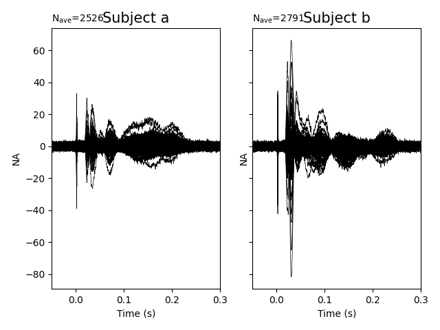
f, axes = plt.subplots(1, 2, sharey=True)
for ax, ev, nc, ll in zip(axes.ravel(), evokeds, noise_covs, ["a", "b"]):
picks = mne.pick_types(ev.info, meg="grad")
ev.plot(picks=picks, axes=ax, noise_cov=nc, show=False)
ax.set_title("Subject %s" % ll, fontsize=15)
plt.show()
del epochs_s
Out:
Opening raw data file /home/circleci/mne_data/HF_SEF/MEG/subject_a/sef_right_raw.fif...
    Read a total of 8 projection items:
        generated with autossp-1.0.1 (1 x 306)  idle
        generated with autossp-1.0.1 (1 x 306)  idle
        generated with autossp-1.0.1 (1 x 306)  idle
        generated with autossp-1.0.1 (1 x 306)  idle
        generated with autossp-1.0.1 (1 x 306)  idle
        generated with autossp-1.0.1 (1 x 306)  idle
        generated with autossp-1.0.1 (1 x 306)  idle
        generated with autossp-1.0.1 (1 x 306)  idle
    Range : 26000 ... 1735999 =      8.667 ...   578.666 secs
Ready.
Opening raw data file /home/circleci/mne_data/HF_SEF/MEG/subject_a/sef_right_raw-1.fif...
    Read a total of 8 projection items:
        generated with autossp-1.0.1 (1 x 306)  idle
        generated with autossp-1.0.1 (1 x 306)  idle
        generated with autossp-1.0.1 (1 x 306)  idle
        generated with autossp-1.0.1 (1 x 306)  idle
        generated with autossp-1.0.1 (1 x 306)  idle
        generated with autossp-1.0.1 (1 x 306)  idle
        generated with autossp-1.0.1 (1 x 306)  idle
        generated with autossp-1.0.1 (1 x 306)  idle
    Range : 1736000 ... 2482999 =    578.667 ...   827.666 secs
Ready.
Current compensation grade : 0
2527 events found
Event IDs: [1]
2527 matching events found
Applying baseline correction (mode: mean)
Not setting metadata
Created an SSP operator (subspace dimension = 8)
8 projection items activated
Opening raw data file /home/circleci/mne_data/HF_SEF/MEG/subject_b/hf_sef_15min_raw.fif...
    Read a total of 8 projection items:
        generated with autossp-1.0.1 (1 x 306)  idle
        generated with autossp-1.0.1 (1 x 306)  idle
        generated with autossp-1.0.1 (1 x 306)  idle
        generated with autossp-1.0.1 (1 x 306)  idle
        generated with autossp-1.0.1 (1 x 306)  idle
        generated with autossp-1.0.1 (1 x 306)  idle
        generated with autossp-1.0.1 (1 x 306)  idle
        generated with autossp-1.0.1 (1 x 306)  idle
    Range : 169000 ... 1878999 =     56.333 ...   626.333 secs
Ready.
Opening raw data file /home/circleci/mne_data/HF_SEF/MEG/subject_b/hf_sef_15min_raw-1.fif...
    Read a total of 8 projection items:
        generated with autossp-1.0.1 (1 x 306)  idle
        generated with autossp-1.0.1 (1 x 306)  idle
        generated with autossp-1.0.1 (1 x 306)  idle
        generated with autossp-1.0.1 (1 x 306)  idle
        generated with autossp-1.0.1 (1 x 306)  idle
        generated with autossp-1.0.1 (1 x 306)  idle
        generated with autossp-1.0.1 (1 x 306)  idle
        generated with autossp-1.0.1 (1 x 306)  idle
    Range : 1879000 ... 2892999 =    626.333 ...   964.333 secs
Ready.
Current compensation grade : 0
2792 events found
Event IDs: [1]
2792 matching events found
Applying baseline correction (mode: mean)
Not setting metadata
Created an SSP operator (subspace dimension = 8)
8 projection items activated
Loading data for 100 events and 1051 original time points ...
0 bad epochs dropped
Computing rank from data with rank=None
    Using tolerance 6.1e-09 (2.2e-16 eps * 306 dim * 8.9e+04  max singular value)
    Estimated rank (mag + grad): 298
    MEG: rank 298 computed from 306 data channels with 8 projectors
    Created an SSP operator (subspace dimension = 8)
    Setting small MEG eigenvalues to zero (without PCA)
Reducing data rank from 306 -> 298
Estimating covariance using EMPIRICAL
Done.
Number of samples used : 15100
[done]
Loading data for 100 events and 1051 original time points ...
0 bad epochs dropped
Computing rank from data with rank=None
    Using tolerance 5.3e-09 (2.2e-16 eps * 306 dim * 7.8e+04  max singular value)
    Estimated rank (mag + grad): 298
    MEG: rank 298 computed from 306 data channels with 8 projectors
    Created an SSP operator (subspace dimension = 8)
    Setting small MEG eigenvalues to zero (without PCA)
Reducing data rank from 306 -> 298
Estimating covariance using EMPIRICAL
Done.
Number of samples used : 15100
[done]
Computing rank from covariance with rank=None
    Using tolerance 1.9e-13 (2.2e-16 eps * 204 dim * 4.1  max singular value)
    Estimated rank (grad): 201
    GRAD: rank 201 computed from 204 data channels with 3 projectors
Computing rank from covariance with rank=None
    Using tolerance 1.2e-14 (2.2e-16 eps * 102 dim * 0.52  max singular value)
    Estimated rank (mag): 97
    MAG: rank 97 computed from 102 data channels with 5 projectors
Computing rank from covariance with rank=None
    Using tolerance 3.3e-13 (2.2e-16 eps * 204 dim * 7.4  max singular value)
    Estimated rank (grad): 201
    GRAD: rank 201 computed from 204 data channels with 3 projectors
Computing rank from covariance with rank=None
    Using tolerance 8e-15 (2.2e-16 eps * 102 dim * 0.35  max singular value)
    Estimated rank (mag): 97
    MAG: rank 97 computed from 102 data channels with 5 projectors
Source and forward modeling
To guarantee an alignment across subjects, we start by computing the source space of fsaverage
resolution = 5
spacing = "oct%d" % resolution

fsaverage_fname = op.join(subjects_dir, "fsaverage")
if not op.exists(fsaverage_fname):
    mne.datasets.fetch_fsaverage(subjects_dir)
src_ref = mne.setup_source_space(subject="fsaverage",
                                 spacing=spacing,
                                 subjects_dir=subjects_dir,
                                 add_dist=False)
Out:
Setting up the source space with the following parameters:

SUBJECTS_DIR = /home/circleci/mne_data/HF_SEF/subjects/
Subject      = fsaverage
Surface      = white
Octahedron subdivision grade 5

>>> 1. Creating the source space...

Doing the octahedral vertex picking...
Loading /home/circleci/mne_data/HF_SEF/subjects/fsaverage/surf/lh.white...
Mapping lh fsaverage -> oct (5) ...
    Warning: zero size triangles: [3 4]
    Triangle neighbors and vertex normals...
Loading geometry from /home/circleci/mne_data/HF_SEF/subjects/fsaverage/surf/lh.sphere...
Setting up the triangulation for the decimated surface...
loaded lh.white 1026/163842 selected to source space (oct = 5)

Loading /home/circleci/mne_data/HF_SEF/subjects/fsaverage/surf/rh.white...
Mapping rh fsaverage -> oct (5) ...
    Warning: zero size triangles: [3 4]
    Triangle neighbors and vertex normals...
Loading geometry from /home/circleci/mne_data/HF_SEF/subjects/fsaverage/surf/rh.sphere...
Setting up the triangulation for the decimated surface...
loaded rh.white 1026/163842 selected to source space (oct = 5)

You are now one step closer to computing the gain matrix
Compute forward models with a reference source space
the function compute_fwd morphs the source space src_ref to the surface of each subject by mapping the sulci and gyri patterns and computes their forward operators. Next we prepare the forward operators to be aligned across subjects
subjects = ["subject_a", "subject_b"]
trans_fname_s = [meg_path + "%s/sef-trans.fif" % s for s in subjects]
bem_fname_s = [subjects_dir + "%s/bem/%s-5120-bem-sol.fif" % (s, s)
               for s in subjects]
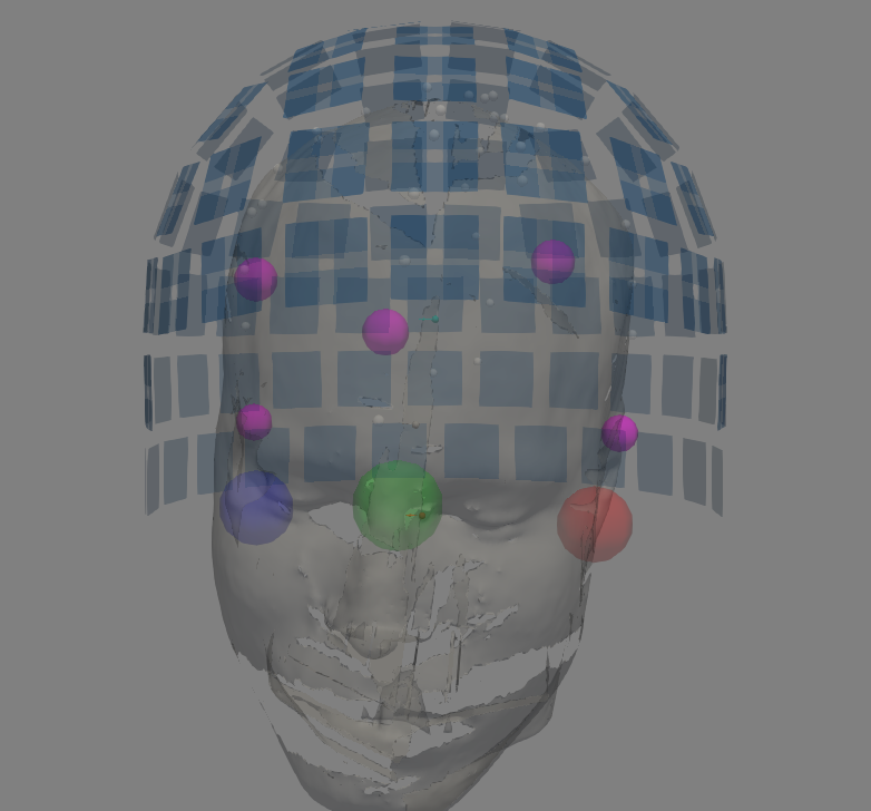
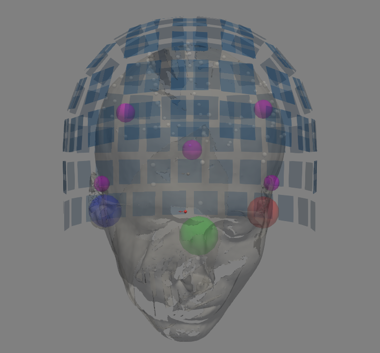
Before computing the forward operators, we make sure the coordinate transformation of the trans file provides a reasonable alignement between the different coordinate systems MEG <-> HEAD
for raw_fname, trans, subject in zip(raw_name_s, trans_fname_s, subjects):
    raw = raw = mne.io.read_raw_fif(raw_fname)
    fig = mne.viz.plot_alignment(raw.info, trans=trans, subject=subject,
                                 subjects_dir=subjects_dir,
                                 surfaces='head-dense',
                                 show_axes=True, dig=True, eeg=[],
                                 meg='sensors',
                                 coord_frame='meg')

n_jobs = 2
parallel, run_func, _ = parallel_func(compute_fwd, n_jobs=n_jobs)


fwds_ = parallel(run_func(s, src_ref, info, trans, bem,  mindist=3)
                 for s, info, trans, bem in zip(subjects, raw_name_s,
                                                trans_fname_s, bem_fname_s))

fwds = prepare_fwds(fwds_, src_ref, copy=False)
Out:
Opening raw data file /home/circleci/mne_data/HF_SEF/MEG/subject_a/sef_right_raw.fif...
    Read a total of 8 projection items:
        generated with autossp-1.0.1 (1 x 306)  idle
        generated with autossp-1.0.1 (1 x 306)  idle
        generated with autossp-1.0.1 (1 x 306)  idle
        generated with autossp-1.0.1 (1 x 306)  idle
        generated with autossp-1.0.1 (1 x 306)  idle
        generated with autossp-1.0.1 (1 x 306)  idle
        generated with autossp-1.0.1 (1 x 306)  idle
        generated with autossp-1.0.1 (1 x 306)  idle
    Range : 26000 ... 1735999 =      8.667 ...   578.666 secs
Ready.
Opening raw data file /home/circleci/mne_data/HF_SEF/MEG/subject_a/sef_right_raw-1.fif...
    Read a total of 8 projection items:
        generated with autossp-1.0.1 (1 x 306)  idle
        generated with autossp-1.0.1 (1 x 306)  idle
        generated with autossp-1.0.1 (1 x 306)  idle
        generated with autossp-1.0.1 (1 x 306)  idle
        generated with autossp-1.0.1 (1 x 306)  idle
        generated with autossp-1.0.1 (1 x 306)  idle
        generated with autossp-1.0.1 (1 x 306)  idle
        generated with autossp-1.0.1 (1 x 306)  idle
    Range : 1736000 ... 2482999 =    578.667 ...   827.666 secs
Ready.
Current compensation grade : 0
Using subject_a-head-dense.fif for head surface.
    1 BEM surfaces found
    Reading a surface...
[done]
    1 BEM surfaces read
Using pyvista 3d backend.

Opening raw data file /home/circleci/mne_data/HF_SEF/MEG/subject_b/hf_sef_15min_raw.fif...
    Read a total of 8 projection items:
        generated with autossp-1.0.1 (1 x 306)  idle
        generated with autossp-1.0.1 (1 x 306)  idle
        generated with autossp-1.0.1 (1 x 306)  idle
        generated with autossp-1.0.1 (1 x 306)  idle
        generated with autossp-1.0.1 (1 x 306)  idle
        generated with autossp-1.0.1 (1 x 306)  idle
        generated with autossp-1.0.1 (1 x 306)  idle
        generated with autossp-1.0.1 (1 x 306)  idle
    Range : 169000 ... 1878999 =     56.333 ...   626.333 secs
Ready.
Opening raw data file /home/circleci/mne_data/HF_SEF/MEG/subject_b/hf_sef_15min_raw-1.fif...
    Read a total of 8 projection items:
        generated with autossp-1.0.1 (1 x 306)  idle
        generated with autossp-1.0.1 (1 x 306)  idle
        generated with autossp-1.0.1 (1 x 306)  idle
        generated with autossp-1.0.1 (1 x 306)  idle
        generated with autossp-1.0.1 (1 x 306)  idle
        generated with autossp-1.0.1 (1 x 306)  idle
        generated with autossp-1.0.1 (1 x 306)  idle
        generated with autossp-1.0.1 (1 x 306)  idle
    Range : 1879000 ... 2892999 =    626.333 ...   964.333 secs
Ready.
Current compensation grade : 0
Using subject_b-head-dense.fif for head surface.
    1 BEM surfaces found
    Reading a surface...
[done]
    1 BEM surfaces read
[Parallel(n_jobs=2)]: Using backend LokyBackend with 2 concurrent workers.
[Parallel(n_jobs=2)]: Done   2 out of   2 | elapsed:   33.9s remaining:    0.0s
[Parallel(n_jobs=2)]: Done   2 out of   2 | elapsed:   33.9s finished
Mapping lh fsaverage -> subject_a (nearest neighbor)...
Mapping rh fsaverage -> subject_a (nearest neighbor)...
Mapping lh fsaverage -> subject_b (nearest neighbor)...
Mapping rh fsaverage -> subject_b (nearest neighbor)...
Solve the inverse problems with Multi-task Lasso
# The Multi-task Lasso assumes the source locations are the same across
# subjects for all instants i.e if a source is zero for one subject, it will
# be zero for all subjects. "alpha" is a hyperparameter that controls this
# structured sparsity prior. it must be set as a positive number between 0
# and 1. With alpha = 1, all the sources are 0.

# We restric the time points around 20ms in order to reconstruct the sources of
# the N20 response.
evokeds = [ev.crop(0.019, 0.021) for ev in evokeds]

stcs = compute_group_inverse(fwds, evokeds, noise_covs,
                             method='multitasklasso',
                             spatiotemporal=True,
                             alpha=0.8)
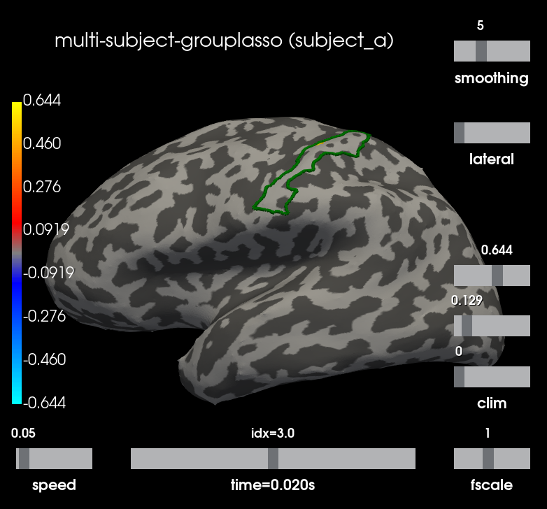
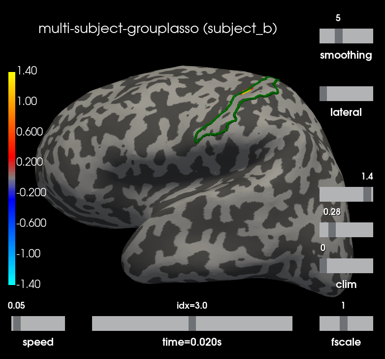
Let’s visualize the N20 response. The stimulus was applied on the right hand, thus we only show the left hemisphere. The activation is exactly in the primary somatosensory cortex. We highlight the borders of the post central gyrus.
t = 0.02
plot_kwargs = dict(
    hemi='lh', subjects_dir=subjects_dir, views="lateral",
    initial_time=t, time_unit='s', size=(800, 800),
    smoothing_steps=5)

t_idx = stcs[0].time_as_index(t)

for stc, subject in zip(stcs, subjects):
    g_post_central = mne.read_labels_from_annot(subject, "aparc.a2009s",
                                                subjects_dir=subjects_dir,
                                                regexp="G_postcentral-lh")[0]
    n_sources = [stc.vertices[0].size, stc.vertices[1].size]
    m = abs(stc.data[:n_sources[0], t_idx]).max()
    plot_kwargs["clim"] = dict(kind='value', pos_lims=[0., 0.2 * m, m])
    brain = stc.plot(**plot_kwargs)
    brain.add_text(0.1, 0.9, "multi-subject-grouplasso (%s)" % subject,
                   "title")
    brain.add_label(g_post_central, borders=True, color="green")
Out:
Reading labels from parcellation...
   read 1 labels from /home/circleci/mne_data/HF_SEF/subjects/subject_a/label/lh.aparc.a2009s.annot
   read 0 labels from /home/circleci/mne_data/HF_SEF/subjects/subject_a/label/rh.aparc.a2009s.annot
Reading labels from parcellation...
   read 1 labels from /home/circleci/mne_data/HF_SEF/subjects/subject_b/label/lh.aparc.a2009s.annot
   read 0 labels from /home/circleci/mne_data/HF_SEF/subjects/subject_b/label/rh.aparc.a2009s.annot
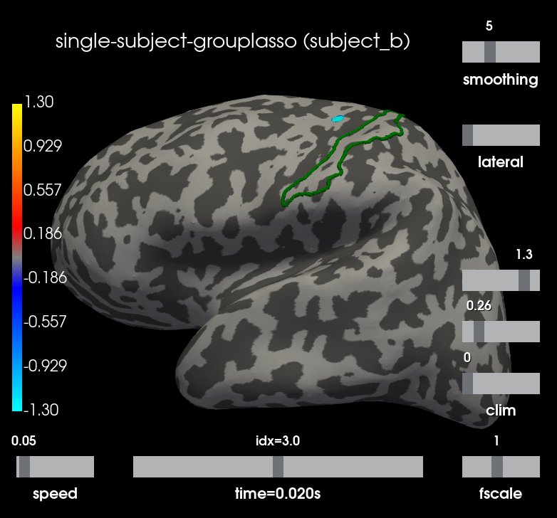
Group MNE leads to better accuracy
To evaluate the effect of the joint inverse solution, we compute the individual solutions independently for each subject
for subject, fwd, evoked, cov in zip(subjects, fwds_, evokeds, noise_covs):
    fwd_ = prepare_fwds([fwd], src_ref)
    stc = compute_group_inverse(fwd_, [evoked], [cov],
                                method='multitasklasso',
                                spatiotemporal=True,
                                alpha=0.8)[0]
    stc.subject = subject
    g_post_central = mne.read_labels_from_annot(subject, "aparc.a2009s",
                                                subjects_dir=subjects_dir,
                                                regexp="G_postcentral-lh")[0]
    n_sources = [stc.vertices[0].size, stc.vertices[1].size]
    m = abs(stc.data[:n_sources[0], t_idx]).max()
    plot_kwargs["clim"] = dict(kind='value', pos_lims=[0., 0.2 * m, m])
    brain = stc.plot(**plot_kwargs)
    brain.add_text(0.1, 0.9, "single-subject-grouplasso (%s)" % subject,
                   "title")
    brain.add_label(g_post_central, borders=True, color="green")

Out:
Mapping lh fsaverage -> subject_a (nearest neighbor)...
Mapping rh fsaverage -> subject_a (nearest neighbor)...
Reading labels from parcellation...
   read 1 labels from /home/circleci/mne_data/HF_SEF/subjects/subject_a/label/lh.aparc.a2009s.annot
   read 0 labels from /home/circleci/mne_data/HF_SEF/subjects/subject_a/label/rh.aparc.a2009s.annot
Mapping lh fsaverage -> subject_b (nearest neighbor)...
Mapping rh fsaverage -> subject_b (nearest neighbor)...
Reading labels from parcellation...
   read 1 labels from /home/circleci/mne_data/HF_SEF/subjects/subject_b/label/lh.aparc.a2009s.annot
   read 0 labels from /home/circleci/mne_data/HF_SEF/subjects/subject_b/label/rh.aparc.a2009s.annot
References
[1] Michael Lim, Justin M. Ales, Benoit R. Cottereau, Trevor Hastie, Anthony M. Norcia. Sparse EEG/MEG source estimation via a group lasso, PLOS ONE, 2017
[2] Jussi Nurminen, Hilla Paananen, & Jyrki Mäkelä. (2017). High frequency somatosensory MEG: evoked responses, FreeSurfer reconstruction [Data set]. Zenodo. http://doi.org/10.5281/zenodo.889235
Total running time of the script: ( 3 minutes 17.695 seconds)
Estimated memory usage: 1021 MB