MTW Handwritten Digits Classification

This example performs classification of Handwritten digits using MTW. Each digit recognition is learned as a sparse regression task. This example can be used to reproduce the results of (Janati et al., Aistats‘19).

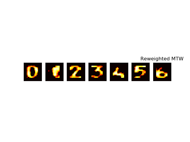
Reweighting reduces the bias amplitude and highlights the sharp features.

import numpy as np
import os
from download import download

from mutar import ReMTW, MTW, utils

from matplotlib import pyplot as plt

print(__doc__)

seed = 42
rnd = np.random.RandomState(seed)

# set n_samples
n_samples = 30
n_features = 240

# take only 3 tasks to run example fast
tasks = [0, 1, 2, 3, 4, 5, 6]
n_tasks = len(tasks)
mtgl_only = False
positive = False

Out:

Download data. The images ‘X’ are grouped and sorted. Generate true labels ‘Y’ accordingly

if not os.path.exists('./data'):
    os.mkdir('./data')
url = "http://archive.ics.uci.edu/ml/machine-learning-databases/"
url += "mfeat/mfeat-pix"

if not os.path.exists(".data/digits.txt"):
    path = download(url, ".data/digits.txt", replace=True)
Xraw = np.loadtxt(".data/digits.txt")
Xraw = Xraw.reshape(10, 200, 240)
yraw = np.zeros((10, 2000))
for k in range(10):
    yraw[k, 200 * k: 200 * (k + 1)] = 1.
yraw = yraw.reshape(10, 10, 200)

Each digit corresponds to a task. Reshape data to fit a multi-task learner and split it into a cv and validation set. Here the design matrix X is the same for all tasks.”“”

samples = np.arange(200)
samples = rnd.permutation(samples)[:n_samples]
mask_valid = np.ones(200).astype(bool)
mask_valid[samples] = False
ycv = yraw[tasks][:, tasks][:, :, samples].reshape(n_tasks, -1)
yvalid = yraw[tasks][:, tasks][:, :, mask_valid].reshape(n_tasks, -1)
yvalid = np.argmax(yvalid, axis=0)
Xvalid = Xraw[tasks][:, mask_valid].reshape(-1, n_features)
X = Xraw[tasks][:, samples]
X = X.reshape(n_tasks * n_samples, n_features)
scaling = X.std(axis=0)
scaling[scaling == 0] = 1
X = X / scaling
Xcv = np.array(n_tasks * [X])

Compute a Euclidean Ground metric M on a 2D grid.

x = np.arange(16).reshape(-1, 1).astype(float)
y = np.arange(15).reshape(-1, 1).astype(float)

xx, yy = np.meshgrid(x, y)
M1 = abs(xx - yy) ** 2
M = M1[:, np.newaxis, :, np.newaxis] + M1[np.newaxis, :, np.newaxis, :]
M = M.reshape(n_features, n_features) ** 0.5
M_ = M ** 2
M_ /= np.median(M_)

Create an MTW instance and fit

epsilon = 1. / n_features
betamax = np.array([abs(x.T.dot(y)) for x, y in zip(Xcv, ycv)]).max()
alpha = 0.5
beta = 0.2 * betamax / n_samples
gamma = utils.compute_gamma(0.9, M_)
mtw = MTW(M=M_, alpha=alpha, beta=beta, epsilon=epsilon, gamma=gamma,
          normalize=False)

mtw.fit(Xcv, ycv)

coefs_ = mtw.coef_.copy()
ypred = np.argmax(Xvalid.dot(coefs_), axis=1)
errors = (ypred != yvalid).reshape(n_tasks, -1).mean(axis=1)

print(f"Classification error for predicting digits {tasks}:")
print(errors)

Out:

Classification error for predicting digits [0, 1, 2, 3, 4, 5, 6]:
[0.01176471 0.06470588 0.02941176 0.18235294 0.58235294 0.14117647
 0.15882353]

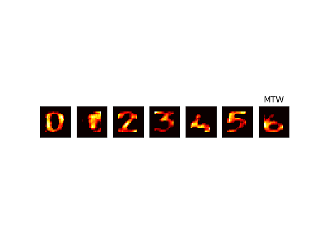
Imshow coefficients

largecoef = np.zeros((n_tasks, 24, 24))
coefs_ = mtw.coef_.copy()
# coefs_ /= coefs_.max(axis=0)[None, :]
coefs_ = np.clip(coefs_, 0, None)
c = coefs_.reshape(16, 15, n_tasks)
c = np.swapaxes(c, 0, 2)
largecoef[:, 4:19][:, :, 4:20] = c

f, axes = plt.subplots(1, n_tasks)
for ax, coef in zip(axes.T, largecoef):
    ax.imshow(np.log(coef.T + 0.1), cmap="hot")
    ax.set_xticks([])
    ax.set_yticks([])
plt.title("MTW")
plt.show()

Do the same thing with Reweighted MTW

mtw = ReMTW(M=M_, alpha=alpha, beta=beta, epsilon=epsilon, gamma=gamma,
            tol_reweighting=1e-6)
mtw.fit(Xcv, ycv)
coefs_ = mtw.coef_.copy()

ypred = np.argmax(Xvalid.dot(coefs_), axis=1)
errors = (ypred != yvalid).reshape(n_tasks, -1).mean(axis=1)

print(f"Classification error for predicting digits {tasks}:")
print(errors)

Out:

Classification error for predicting digits [0, 1, 2, 3, 4, 5, 6]:
[0.01176471 0.06470588 0.04705882 0.24117647 0.64117647 0.17058824
 0.18235294]

Imshow coefficients

largecoef = np.zeros((n_tasks, 24, 24))
coefs_ = mtw.coef_.copy()
coefs_ /= coefs_.max(axis=0)[None, :]
coefs_ = np.clip(coefs_, 0, None)
c = coefs_.reshape(16, 15, n_tasks)
c = np.swapaxes(c, 0, 2)
largecoef[:, 4:19][:, :, 4:20] = c

f, axes = plt.subplots(1, n_tasks)
for ax, coef in zip(axes.T, largecoef):
    ax.imshow(np.log(coef.T + 0.1), cmap="hot")
    ax.set_xticks([])
    ax.set_yticks([])
plt.title("Reweighted MTW")
plt.show()

Estimated memory usage: 28 MB